Avoiding local optima
Giulio Barcaroli
2026-10-22
Source:vignettes/local_optima.Rmd
local_optima.RmdWhy the QGA gets stuck
Like most evolutionary algorithms, the QGA can converge prematurely to a local optimum. In the QGA this happens for three reasons:
All individuals follow the same attractor. At each generation the rotation gate moves the qubits of every individual towards the best individual of the generation. After a few generations the population becomes homogeneous, and the search continues only around that solution.
Qubits saturate. When the probability of a bit value approaches 0 or 1, the measurement becomes deterministic. Near these extremes the rotation changes the probability very little, so the bit is practically frozen.
A large rotation angle accelerates convergence.
thetais the step by which every qubit is rotated towards the best solution: a largethetadoes not mean more exploration, but faster collapse on the first good solution found. Exploration comes from keeping the qubits in superposition.
Mutation and interference do not solve the problem: mutation acts on very few qubits, and interference only redistributes the diversity that is already in the population, without creating new diversity.
The QGA function offers some parameters to counteract
premature convergence. They are all switched off by default, so that the
standard behaviour is unchanged.
A deceptive test problem
To show their effect we use a deceptive trap function: the solution is made of 12 blocks of 4 bits; the value of each block is 4 if all its bits are 1, otherwise 3 minus the number of ones. The global optimum (all ones) is 48, but each block “pushes” towards all zeros, a local optimum worth 36.
trap4 <- function(solution, eval_func_inputs) {
  bits <- solution - 1                 # QGA values are 1..nvalues_sol
  u <- colSums(matrix(bits, nrow = 4)) # number of ones in each block
  sum(ifelse(u == 4, 4, 3 - u))
}
We run the QGA with the default parameters:
set.seed(1)
base <- QGA(popsize = 20,
            generation_max = 300,
            nvalues_sol = 2,
            Genome = 48,
            eval_fitness = trap4,
            eval_func_inputs = NULL,
            plotting = FALSE,
            verbose = FALSE,
            progress = FALSE)
max(base[[2]]$fitness_best)
#> [1] 44
The parameters
Rotation angle: thetainit and
thetaend
The rotation angle decreases linearly from thetainit to
thetaend. A qubit starts around pi/4 (equal probabilities)
and becomes deterministic at 0 or pi/2: if it is always pushed in the
same direction, it saturates after about (pi/4)/theta generations.
| theta | generations_to_saturate |
|---|---|
| 0.05*pi | 5 |
| 0.025*pi | 10 |
| 0.01*pi | 25 |
| 0.005*pi | 50 |
| 0.001*pi | 250 |
With the default values (thetainit = 0.05*pi,
thetaend = 0.025*pi) a bit can be decided in 5 to 10
generations. As a rule of thumb, choose theta so that
saturation requires at least 10-20% of generation_max, for
instance thetainit = 0.01*pi and
thetaend = 0.005*pi with 200-300 generations. Smaller
values slow down convergence, so more generations may be needed.
H-epsilon gate: epsilon
The H-epsilon gate (Han and Kim, 2004) keeps the probability of each
bit value in [epsilon, 1 - epsilon], so that
qubits never collapse completely and every bit always keeps a small
probability of changing. Typical values are 0.01-0.05.
QGA(..., epsilon = 0.02)In our experiments the gate alone did not improve the results: with small values it acts like a light mutation. It can be useful in combination with the other options.
Partial restart: restart_iters and
restart_strength
When the best fitness does not improve for restart_iters
generations, the population is partially brought back towards equal
probabilities: the angle of each qubit is moved towards pi/4 by the
fraction restart_strength (0 = no change, 1 = complete
reset). The individual equal to the best solution is preserved, so
nothing already found is lost. After a restart the counter starts
again.
set.seed(1)
restart <- QGA(popsize = 20,
               generation_max = 300,
               nvalues_sol = 2,
               Genome = 48,
               eval_fitness = trap4,
               eval_func_inputs = NULL,
               plotting = FALSE,
               verbose = FALSE,
               progress = FALSE,
               restart_iters = 20,
               restart_strength = 0.5)
max(restart[[2]]$fitness_best)
#> [1] 48
If stop_iters is used, restart_iters must
be smaller than stop_iters, otherwise the algorithm stops
before any restart.
Choosing restart_iters and
restart_strength
The benchmark below (20 seeds for each configuration,
popsize = 20, default theta; see the last
section for the two problems) shows that the good values of
restart_iters do not scale with
generation_max: they depend on the time a qubit needs to
saturate, about (pi/4)/theta generations (see the table on
theta above). With the default angles this time is 5-10
generations, and on trap-4 restart_iters = 20 finds the
optimum in 20 runs out of 20 with 600 generations, while
restart_iters = 40 never does, with 300 or 600 generations.
Frequent restarts work because the population never collapses
completely: every restart pushes it back in superposition before the
qubits freeze.
| generation_max | restart_iters | restart_strength | trap4_mean | trap4_optimum_found | rastrigin_mean |
|---|---|---|---|---|---|
| 300 | none | 42.25 | 0/20 | -11.31 | |
| 300 | 10 | 0.25 | 46.50 | 14/20 | -11.72 |
| 300 | 10 | 0.5 | 48.00 | 20/20 | -15.58 |
| 300 | 10 | 1 | 40.90 | 1/20 | -19.99 |
| 300 | 20 | 0.25 | 42.30 | 0/20 | -11.00 |
| 300 | 20 | 0.5 | 46.20 | 12/20 | -10.69 |
| 300 | 20 | 1 | 43.20 | 3/20 | -14.07 |
| 300 | 40 | 0.25 | 42.25 | 0/20 | -11.27 |
| 300 | 40 | 0.5 | 42.20 | 0/20 | -10.21 |
| 300 | 40 | 1 | 42.80 | 1/20 | -11.36 |
| 300 | 80 | 0.25 | 42.25 | 0/20 | -11.16 |
| 300 | 80 | 0.5 | 42.25 | 0/20 | -11.24 |
| 300 | 80 | 1 | 42.25 | 0/20 | -10.08 |
| 150 | none | 42.20 | 0/20 | -12.39 | |
| 150 | 5 | 0.5 | 37.10 | 5/20 | -27.75 |
| 150 | 10 | 0.5 | 45.40 | 14/20 | -19.75 |
| 150 | 20 | 0.5 | 42.10 | 0/20 | -13.09 |
| 150 | 40 | 0.5 | 42.20 | 0/20 | -12.77 |
| 600 | none | 42.25 | 0/20 | -9.16 | |
| 600 | 20 | 0.5 | 48.00 | 20/20 | -9.98 |
| 600 | 40 | 0.5 | 42.30 | 0/20 | -8.45 |
| 600 | 80 | 0.5 | 42.25 | 0/20 | -9.17 |
| 600 | 160 | 0.5 | 42.25 | 0/20 | -9.33 |
From these results:
-
restart_strength: 0.5 is the best compromise. A complete reset (1) throws away what the population has learned and is equivalent to a random restart; a weak restart (0.25) helps only if it is very frequent. -
restart_iters: on a deceptive problem, take 1.5-3 times the saturation time, i.e. 10-20 with the default angles, and proportionally more with smaller angles (for instance 40-80 withthetainit = 0.01*pi). On a problem with many local optima, like Rastrigin, frequent restarts are harmful (they interrupt the local search), and less frequent restarts (40-80) give at most a small improvement. -
generation_max: it does not determinerestart_iters, but it must leave room for several restarts after the population has converged: with 150 generations evenrestart_iters = 10is less effective than with 300. As a rough rule,generation_maxshould be at least 10-15 timesrestart_iters.
Restoring the rotation angle: restart_theta
Since theta decays during the run, a late restart works
with a small angle. With restart_theta = TRUE, at each
restart theta is brought back to thetainit and
decays again to thetaend over the remaining
generations.
| generation_max | restart_iters | restart_strength | trap4_found_FALSE | trap4_found_TRUE | rastrigin_FALSE | rastrigin_TRUE |
|---|---|---|---|---|---|---|
| 300 | 20 | 0.5 | 12/20 | 1/20 | -10.69 | -10.39 |
| 300 | 20 | 1.0 | 3/20 | 10/20 | -14.07 | -13.16 |
| 300 | 40 | 0.5 | 0/20 | 0/20 | -10.21 | -9.57 |
| 300 | 40 | 1.0 | 1/20 | 2/20 | -11.36 | -10.10 |
| 150 | 10 | 0.5 | 14/20 | 18/20 | -19.75 | -16.88 |
| 150 | 20 | 0.5 | 0/20 | 0/20 | -13.09 | -12.90 |
| 600 | 40 | 0.5 | 0/20 | 0/20 | -8.45 | -7.99 |
| 600 | 80 | 0.5 | 0/20 | 0/20 | -9.17 | -8.84 |
The effect is mixed. On Rastrigin restoring the angle always gives a
slightly better mean, but the differences are small compared with the
variability among seeds. On trap-4 it helps after a complete reset
(restart_strength = 1) and with few generations, but it
spoils the best configuration (restart_iters = 20,
restart_strength = 0.5: from 12/20 to 1/20). The reason is
that theta is the step towards the attractor: right after a
partial restart the attractor is still the best solution, and a larger
angle brings the population back to it more quickly. For this reason
restart_theta is off by default; it can be tried together
with stronger restarts.
Personal attractors and migration:
attractor_type = "personal"
With attractor_type = "personal" (Han and Kim, 2002)
every individual is rotated towards its own attractor, i.e. the best
solution it has found so far, instead of the best individual of the
generation. In this way the population keeps several “niches” of search.
The attractors are shared through migration:
-
migration_group_size(default 2): the population is divided into groups of consecutive individuals; -
migration_local_period(default 1): every this many generations, the best attractor of each group is copied to the other members of the group (local migration); -
migration_global_period(default 50): every this many generations, the best attractor is copied to all individuals (global migration).
Larger groups and more frequent global migration make the search more similar to the standard one; smaller groups and rarer global migration preserve more diversity, but slow down convergence.
set.seed(1)
personal <- QGA(popsize = 20,
                generation_max = 300,
                nvalues_sol = 2,
                Genome = 48,
                eval_fitness = trap4,
                eval_func_inputs = NULL,
                plotting = FALSE,
                verbose = FALSE,
                progress = FALSE,
                attractor_type = "personal")
max(personal[[2]]$fitness_best)
#> [1] 45
Interference: interference_flag,
interference_type, interference_rate,
interference_lambda
The interference operator recombines information among individuals,
with probability interference_rate at each generation:
-
interference_type = "diagonal": the amplitudes of the j-th qubit of each individual are copied from another individual following a diagonal scheme (Narayanan and Moore, 1996); -
interference_type = "amplitude": each qubit receives the sum of the amplitudes of the whole population, weighted by fitness, so that individuals above the average fitness interfere constructively and those below destructively;interference_lambdasets the strength.
Being a recombination operator, interference does not create new diversity, and in our experiments it did not help to escape local optima.
Comparing the runs
plot(base[[2]]$fitness_best, type = "l", ylim = c(30, 48),
     xlab = "generation", ylab = "best fitness")
lines(restart[[2]]$fitness_best, col = "red")
lines(personal[[2]]$fitness_best, col = "blue")
abline(h = 48, lty = 2)
legend("bottomright", lty = 1, col = c("black", "red", "blue"),
       legend = c("default", "restart_iters = 20", "attractor_type = 'personal'"))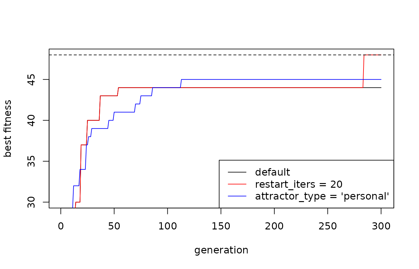
A single run is not enough to compare the options, because the QGA is stochastic. The following section reports the results obtained on 20 runs for each configuration.
Benchmark results
Two problems with known optimum were used, with
popsize = 20, generation_max = 300, 20 seeds
for each configuration, default theta:
- trap-4: the deceptive function above (optimum 48);
- Rastrigin: 6 dimensions, 64 values in [-5.12, 4.96] for each dimension, a function with many local optima (maximum 0).
The column last_improvement is the average generation of
the last improvement of the best fitness: low values mean that the
search stopped early.
| configuration | trap4_mean | trap4_optimum_found | trap4_last_improvement | rastrigin_mean | rastrigin_last_improvement |
|---|---|---|---|---|---|
| default | 42.25 | 0/20 | 64 | -11.31 | 124 |
| epsilon = 0.02 | 41.65 | 0/20 | 49 | -10.76 | 177 |
| restart_iters = 20 | 46.20 | 12/20 | 214 | -10.69 | 96 |
| attractor_type = ‘personal’ | 44.80 | 0/20 | 111 | -7.96 | 221 |
| all three | 43.70 | 0/20 | 130 | -7.25 | 217 |
| personal + restart_iters = 10 | 42.30 | 0/20 | 126 | -11.88 | 192 |
| personal + restart_iters = 20 | 44.50 | 0/20 | 131 | -8.34 | 232 |
| personal + restart_iters = 40 | 44.75 | 0/20 | 116 | -7.67 | 220 |
The main findings are:
- restart is the most effective option on the deceptive problem: it finds the global optimum in 12 runs out of 20, while the default configuration never escapes the trap; on Rastrigin it does not help;
- personal attractors are the only option that improves significantly on both problems; the search goes on until the end of the run, so more generations would probably improve the results further;
- the H-epsilon gate alone does not help;
- combining restart and personal attractors does not add up their advantages: the result is similar to personal attractors alone. A possible explanation is that after a restart the individuals are rotated back towards their old attractors, i.e. towards the same local optima.
Practical recommendations
- Start from smaller rotation angles than the defaults, taking into account the number of generations (see the table above).
- If the fitness history shows a long flat line with an early last
improvement, try a partial restart with
restart_strength = 0.5andrestart_itersequal to 1.5-3 times the saturation time (pi/4)/theta, i.e. 10-20 with the default angles, independently ofgeneration_max. - Use
parameters_hint()to get a first set of values fromgeneration_max, the genome and the kind of problem (see below). - For problems with many local optima scattered in the search space,
try
attractor_type = "personal", possibly with more generations. - Always compare the options on several runs (different seeds), and if
the fitness evaluation is expensive consider
parallel = TRUE.
Suggested values: parameters_hint()
The function parameters_hint() turns the guidelines
above into a first set of values, given generation_max, the
genome (Genome, nvalues_sol) and the kind of
problem ("deceptive", "multimodal",
"unimodal" or "unknown"):
- the angles are chosen so that the saturation time is about
generation_max / 40when restarts are used, andgeneration_max / 10otherwise, never faster than the default angles; -
restart_itersis 1.5 times the saturation time for deceptive problems, 3 times when the problem is unknown, 6 times for problems with many local optima; no restart for unimodal problems; -
restart_strength = 0.5; personal attractors for unknown and multimodal problems.
hint <- parameters_hint(generation_max = 300, Genome = 48, nvalues_sol = 2,
                        problem_type = "deceptive")
#>
#>  QGA parameters hint
#>  -------------------
#>  problem_type: deceptive; genome of 48 genes x 1 bits = 48 qubits; 300 generations
#>  saturation time (pi/4)/theta: about 7.5 generations
#>
#>  thetainit        = 0.1396   (= 0.0444 * pi)
#>  thetaend         = 0.0698   (= 0.0222 * pi)
#>  restart_iters    = 11   (1.5 x saturation time)
#>  restart_strength = 0.5
#>  restart_theta    = FALSE  (experimental)
#>  epsilon          = 0
#>  attractor_type   = "generation"
#>
#>  fitness evaluations: up to 6020
#>  These are starting points: compare a few configurations on several seeds.
The returned list can be passed directly to QGA():
out <- do.call(QGA, c(list(popsize = 20, generation_max = 300,
                           nvalues_sol = 2, Genome = 48,
                           eval_fitness = trap4, eval_func_inputs = NULL),
                      hint))
On the two test problems (20 seeds, popsize = 20) the
suggested values improve on the defaults for every number of
generations, both when the kind of problem is given and when it is
declared unknown:
| generation_max | configuration | trap4_mean | trap4_optimum_found | rastrigin_mean |
|---|---|---|---|---|
| 150 | default | 42.20 | 0/20 | -12.39 |
| 150 | hint (problem type given) | 45.40 | 14/20 | -10.35 |
| 150 | hint (unknown) | 43.95 | 1/20 | -11.21 |
| 300 | default | 42.25 | 0/20 | -11.31 |
| 300 | hint (problem type given) | 48.00 | 20/20 | -9.00 |
| 300 | hint (unknown) | 44.00 | 1/20 | -9.56 |
| 600 | default | 42.25 | 0/20 | -9.16 |
| 600 | hint (problem type given) | 47.60 | 19/20 | -6.02 |
| 600 | hint (unknown) | 43.50 | 0/20 | -6.81 |
Knowing the kind of problem helps, especially on the deceptive one:
with "unknown" the function chooses personal attractors,
which are a good compromise on both problems but are less effective than
restarts alone on trap-4. The suggestions are starting points: compare a
few configurations on several seeds.
Which kind of problem?
- Unimodal: there is a single optimum, i.e. every local optimum is also the global one; starting from any solution, a chain of small improvements (e.g. changing one bit at a time) always leads to the optimum. Typical examples are additive and separable fitness functions, where each gene contributes independently of the others (e.g. the number of bits equal to 1). Real problems are rarely unimodal.
- Multimodal: there are many local optima, solutions that no small change can improve although better solutions exist elsewhere (e.g. Rastrigin). Almost all real combinatorial problems are multimodal (travelling salesman, knapsack with constraints, clustering, hub location), because of the interactions among genes (the value of a gene depends on the others) and of constraints handled with penalties, which split the search space into separate regions.
- Deceptive: a special case of multimodal problem, in which the local optima have larger basins of attraction and partial improvements lead away from the global optimum (Goldberg, 1989): the combinations of a few genes that give on average a higher fitness are not part of the optimal solution. In trap-4, on average it pays to set the bits to 0, but the optimum has all bits equal to 1.
The structure of the fitness function gives the first indications. Independent contributions of the genes suggest a unimodal problem; interactions or penalties a multimodal one. “All or nothing” rewards (a bonus only when a whole group of genes is complete, while intermediate configurations are worth less than the starting one), thresholds and penalties for intermediate states, or an optimum lying on a narrow boundary between constraints, reachable only through infeasible or penalised solutions, are typical signs of deception.
The kind of problem can also be explored empirically:
-
Comparing configurations on 5-10 seeds each (the
simplest and usually sufficient test):
- with the default parameters, if all runs reach the same value and the same solution, the problem is probably unimodal (or at least easy); if they end on different solutions with different values, it is multimodal; if they converge early (low generation of last improvement) and consistently on the same mediocre solution, it may be deceptive;
- if frequent restarts (
problem_type = "deceptive") give a clear jump, as on trap-4 from 42 to 48, the problem is deceptive; - if personal attractors help more than restarts, the problem is rather multimodal.
- Marginal contributions of the genes: on a random sample of solutions, find for each gene the value giving the highest average fitness, and build the corresponding “greedy” solution. If it is poor and differs in many genes from the best solution found by the QGA, the average signal is misleading, i.e. the problem is deceptive. On trap-4 the greedy solution is “all zeros”, worth 36.
- Fitness-distance correlation (Jones and Forrest, 1995): on a sample of solutions, compute the correlation between fitness and Hamming distance from the best known solution. For a maximisation problem a clearly negative correlation (fitness grows when getting closer to the optimum) indicates an easy problem; a correlation close to zero a difficult one; a positive correlation a deceptive one. The optimum must be known: in practice the best solution found is used, with the caveat that it may not be the global one.
"unimodal" removes the restarts and slows down the
rotation, so it should be used only when one is sure: if the problem has
traps, the risk of premature convergence increases. When in doubt, use
"unknown" and switch to "deceptive" or
"multimodal" if the comparison on several seeds suggests
it.
References
- Goldberg, D. E. (1989). Genetic Algorithms in Search, Optimization and Machine Learning. Addison-Wesley.
- Han, K.-H. and Kim, J.-H. (2002). Quantum-inspired evolutionary algorithm for a class of combinatorial optimization. IEEE Transactions on Evolutionary Computation, 6(6), 580-593.
- Han, K.-H. and Kim, J.-H. (2004). Quantum-inspired evolutionary algorithms with a new termination criterion, H-epsilon gate, and two-phase scheme. IEEE Transactions on Evolutionary Computation, 8(2), 156-169.
- Jones, T. and Forrest, S. (1995). Fitness distance correlation as a measure of problem difficulty for genetic algorithms. Proceedings of the Sixth International Conference on Genetic Algorithms, 184-192.
- Narayanan, A. and Moore, M. (1996). Quantum-inspired genetic algorithms. Proceedings of IEEE International Conference on Evolutionary Computation, 61-66.