Maximum of a function

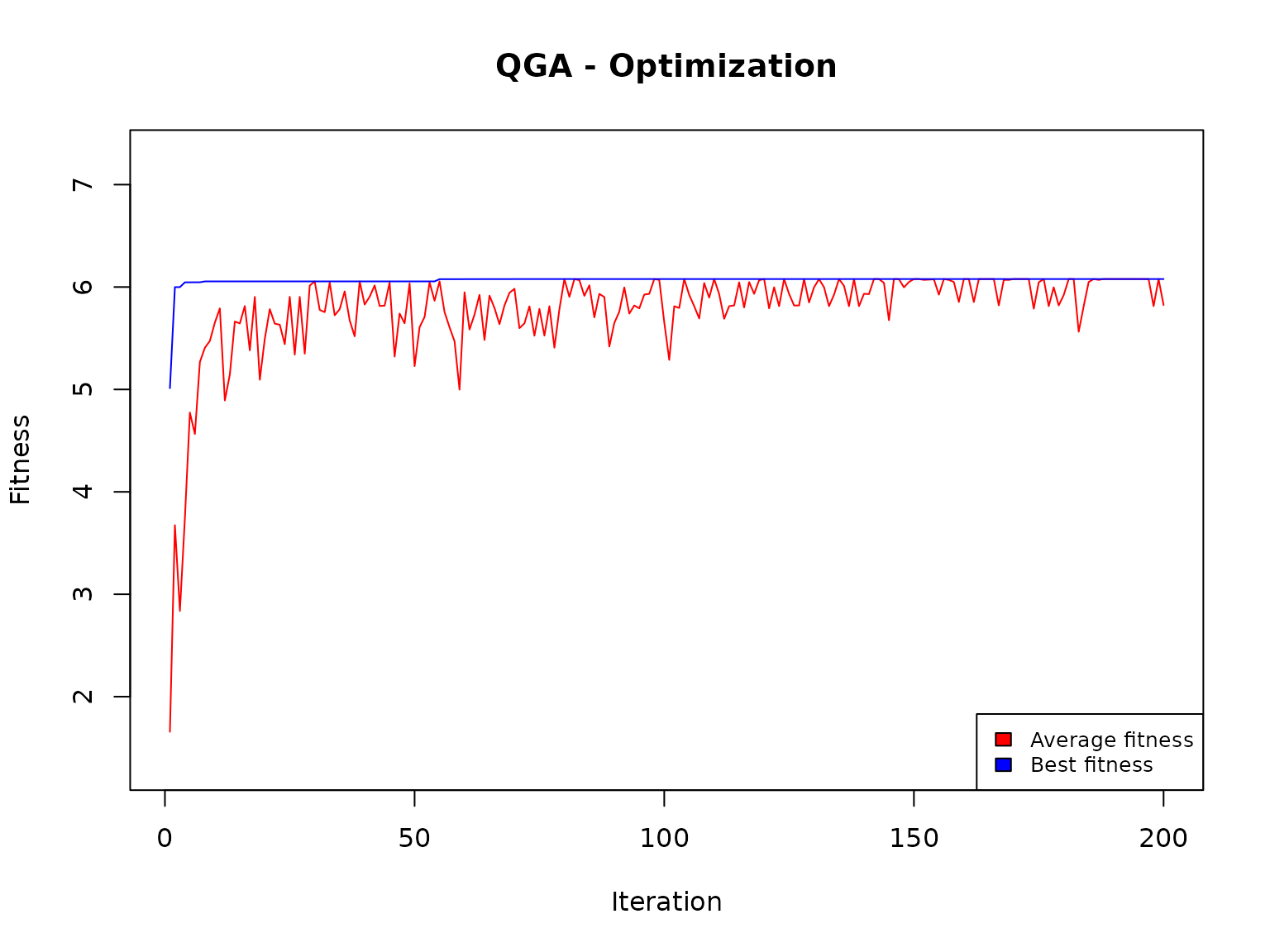
With the Quantum Genetic Algorithm it is possible to determine the maximum (or the minimum) of a function in a given interval of definition.

We consider here the same example reported by Lahoz-Beltra in https://github.com/ResearchCodesHub/QuantumGeneticAlgorithms/blob/master/QGA.py

that is, given a function

f <- function(x) {
  abs((x - 5) / (2 + sin(x)))
}
x <- seq(0,15,0.01)
y <- f(x)
plot(x,y)

we want to determine its maximum in the interval 0-15.

First of all, we use the analytic approach: first, we obtain the first derivative of the function, and then calculate its roots when f(x) = 0:

# Analytic solution
if (!require(numDeriv)) install.packages("numDeriv", dependencies=TRUE)
library(numDeriv)
g <- function(x) {
  (x - 5) / (2 + sin(x))
}
f_prime <- function(x) {
  sgn <- sign(g(x))
  g_deriv <- grad(g, x)
  sgn * g_deriv
}
if (!requireNamespace("rootSolve", quietly = TRUE)) {
  install.packages("rootSolve")
}
library(rootSolve)
root1 <- uniroot(f_prime, c(5.1, 12))$root
root2 <- uniroot(f_prime, c(12.1, 15))$root
# cat("Root 1: x ≈", root1, "\n")
# cat("Root 2: x ≈", root2, "\n")
f_root1 <- f(root1)
# f_root2 <- f(root2)
cat("f(", root1, ") ≈", f_root1, "\n")
#> f( 11.16085 ) ≈ 6.078025
# cat("f(", root2, ") ≈", f_root2, "\n")

So, in correspondence with x=11.16085, we have a maximum for f(x) that is equal to 6.078025.

The solution found by Lahoz-Beltra is 5.999, somehow far from the real optimum, basically because in his example he defines a genome whose length is only 4. This implies that only 2^4=16 points are explored in the interval 0-15.

In our QGA application we define, instead, a much longer genome (with 64 (qu)bits), that allows to explore 65536 points in the same interval.

First, we define the fitness function:

functionMax <- function(solution, eval_func_inputs) {
  solution <- solution - 1
  # translate from binary to decimal value
  x=0
  for (j in c(1:Genome)) {
    x=x+solution[j]*2^(Genome-j)
  }
  # Normalize the obtained x into the interval 0-15
  x=x*16/(2^Genome-1)-1
  # replaces the value of x in the function f(x)
  y= abs((x-5)/(2+sin(x)))
  fitness=y
  # Store the current solution
  X <<- c(X,x)
  Y <<- c(Y,y)
  # cat("\nSolution=",solution,"  x=",x,"  y=",y)
  return(fitness)
}

Note that

the solution is always generated as a sequence of 1 and 2, so it is necessary to reduce it to a sequence of 0 and 1 (solution - 1);
the current binary solution is used to generate a real number in the 0-15 interval.

Incidentally, if we want to find the minimum of the f(x), the fitness function should return (-fitness).

Then, we set the parameters:

popsize = 20
generation_max = 200
Genome = 16
nvalues_sol = 2
thetainit = 3.1415926535 * 0.15
thetaend = 3.1415926535 * 0.015
pop_mutation_rate_init = 1/(popsize + 1)
pop_mutation_rate_end = 1/(popsize + 1)
mutation_rate_init = 1/(popsize + 1)
mutation_rate_end = 1/(popsize + 1)
mutation_flag = TRUE

The population size (popsize) and generations (generation_max) are equal to those reported by Lahoz-Beltra. The genome is a sequence of 16 bits (Genome = 16), binary because nvalues_sol=2. The rotation gate is initially set to 3.1415926535 * 0.15, while towards the end it is reduced to 3.1415926535 * 0.15. This allows to explore at the beginning all the interval 0-15, while at the end the exploration is concentrated around the best solution found so far. The mutation rate (Pauli gate) is always set to 1/(popsize + 1)=0.04761905: this means that at each iteration, about 4.7% of the bit values are swapped.

Finally, we apply the quantum genetic algorithm:

library(QGA)
X <- NULL
Y <- NULL
set.seed(1234)
solutionQGA <- QGA(popsize,
                   generation_max,
                   nvalues_sol,
                   Genome=16,
                   thetainit,
                   thetaend,
                   pop_mutation_rate_init,
                   pop_mutation_rate_end,
                   mutation_rate_init,
                   mutation_rate_end,
                   mutation_flag = TRUE,
                   plotting = FALSE,
                   verbose = FALSE,
                   progress = FALSE,
                   eval_fitness = functionMax,
                   eval_func_inputs = list(X,Y))
#> 
#>  *** Best fitness:  6.077961

The found solution is

solution <- solutionQGA[[1]]
solution <- solution - 1
solution
#>  [1] 1 1 0 0 0 0 1 0 0 1 1 1 1 1 1 1
x=0
for (j in c(1:Genome)) {
  x=x+solution[j]*2^(Genome-j)
  # cat("\n",j," solution[j]:",solution[j],"  2^solution[Genome-j-1]:",2^(Genome-j))
}
x=x*16/(2^Genome-1)-1
y= abs((x-5)/(2+sin(x)))
cat("Function maximum: ",y," at x=",x)
#> Function maximum:  6.077961  at x= 11.15619

We remind that the analytical solution was:

cat("f(", root1, ") ≈", f_root1, "\n")
#> f( 11.16085 ) ≈ 6.078025

very close to the one found by the QGA.

Finally, we can have a picture of the exploration of the interval 0-15 by looking at the following plot:

plot(X,Y,type="h",col="red")
title("f(x)=abs((x-5)/(2+sin(x)))")

Giulio Barcaroli

2024-09-25