Travelling salesman
“The travelling salesperson problem, also known as travelling salesman problem, asks the following question:”Given a list of cities and the distances between each pair of cities, what is the shortest possible route that visits each city exactly once and returns to the origin city?” It is an NP-hard problem in combinatorial optimization, important in theoretical computer science and operations research.” (from Wikipedia).
First, we apply the Quantum Genetic Algorithm, then a classical GA, and compare their results.
Prepare data
An external file with a list of cities (names and coordinates) is read, and a number of them is selected (here, only 9):
cities <- read.csv("TSP_cities.csv")
ncities <- 9
cities <- cities[c(1:ncities),]
cities
#>       city     x     y
#> 1    Turin  7.68 45.06
#> 2    Milan  9.19 45.46
#> 3    Genoa  8.93 44.40
#> 4   Venice 12.33 45.43
#> 5  Bologna 11.34 44.49
#> 6 Florence 11.25 43.76
#> 7  Pescara 13.95 42.31
#> 8     Rome 12.48 41.89
#> 9 Naples 14.24 40.83Fitness evaluation
The following fitness evaluation function is defined:
TravellingSalesman <- function(solution,distance) {
  l = 0.0
  for (i in 2:length(solution)) {
    l = l+distance[solution[i-1], solution[i]]
  }
  # Fitness function
  l = l + distance[solution[1],solution[length(solution)]]
  # Penalization
  penal <- ((nrow(distance)) - length(table(solution)))*sum(distance)/10
  cost <- -(penal+l)
  return(cost)
}
This function receives as input parameters:
- solution (the current solution to be evaluated)
- distance (the matrix of distances between the cities to be visited)
distance <- as.matrix(dist(cities[,c(2:3)]))
distance
#>          1        2        3        4        5        6        7        8        9
#> 1 0.000000 1.562082 1.413542 4.664697 3.704119 3.799329 6.846561 5.752295 7.805543
#> 2 1.562082 0.000000 1.091421 3.140143 2.358686 2.670880 5.707898 4.854791 6.851233
#> 3 1.413542 1.091421 0.000000 3.552591 2.411680 2.406657 5.437693 4.347712 6.398515
#> 4 4.664697 3.140143 3.552591 0.000000 1.365174 1.988794 3.515508 3.543177 4.980773
#> 5 3.704119 2.358686 2.411680 1.365174 0.000000 0.735527 3.400662 2.838943 4.669647
#> 6 3.799329 2.670880 2.406657 1.988794 0.735527 0.000000 3.064719 2.238258 4.186287
#> 7 6.846561 5.707898 5.437693 3.515508 3.400662 3.064719 0.000000 1.528823 1.508145
#> 8 5.752295 4.854791 4.347712 3.543177 2.838943 2.238258 1.528823 0.000000 2.054556
#> 9 7.805543 6.851233 6.398515 4.980773 4.669647 4.186287 1.508145 2.054556 0.000000
Here, the distances have been calculated simply as Euclidean distances: clearly, in more realistic cases they should be calculated based on a road map.
Optimization
We define the Genome parameter as the number of cities; also the number of values is set equal to the number of cities. This means that each solution is a vector of 9 elements, each one with an assigned value from 1 to 9: each couple element/value indicates from which origin city (element) the travelling salesman should go to which destination city (value). In this setting, we do not want to introduce the mutation operator. Moreover, we want to iterate 1000 times, each time considering 20 generated solutions.
popsize = 20
Genome = nrow(cities)
nvalues_sol = nrow(cities)
set.seed(4321)
solutionQGA <- QGA(popsize,
                generation_max = 1000,
                nvalues_sol,
                Genome,
                thetainit = 3.1415926535 * 0.01,
                thetaend = 3.1415926535 * 0.01,
                # pop_mutation_rate_init = 1/(popsize + 1),
                # pop_mutation_rate_end = 1/(popsize + 1),
                # mutation_rate_init = 1/(Genome + 1),
                # mutation_rate_end = 1/(Genome + 1),
                mutation_flag = FALSE,
                plotting = FALSE,
                verbose = FALSE,
                progress = FALSE,
                eval_fitness = TravellingSalesman,
                eval_func_inputs = distance,
                stop_iters = 500)
QGA:::plot_Output(solutionQGA[[2]])
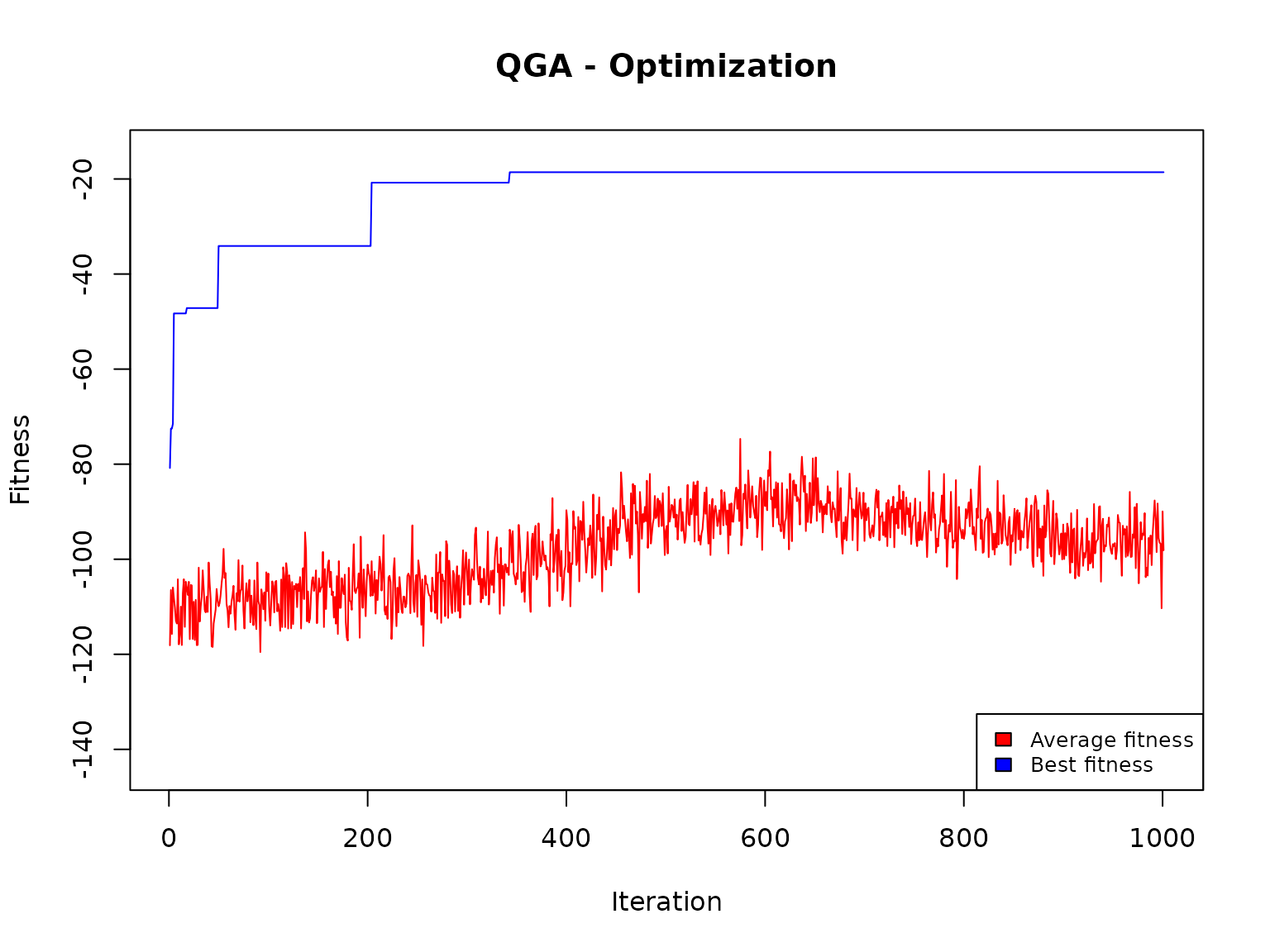
The plot indicates that the number of iterations was enough to obtain a solution that is likely to be no further improved.
Analysis of the solution
solution <- solutionQGA[[1]]
cities$city[solution]
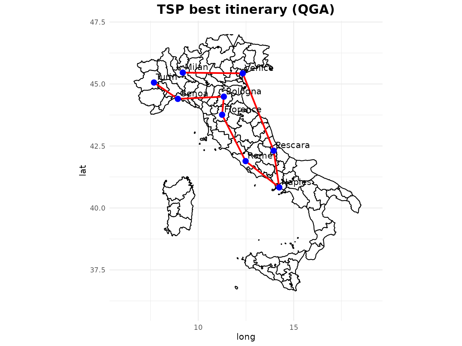
#> [1] "Milan"    "Venice"   "Pescara"  "Naples"   "Rome"     "Florence" "Bologna"  "Genoa"    "Turin"
cities_tsp <- cities[solution,]
The sum of distances:
l = 0.0
for (i in 2:length(solution)) {
  l = l+distance[solution[i-1], solution[i]]
}
l = l + distance[solution[1],solution[length(solution)]]
l
#> [1] 18.57944
# Plot
if (!require(maps)) install.packages("maps")
if (!require(tidyverse)) install.packages("tidyverse")
if (!require(ggplot2)) install.packages("ggplot2")
library(maps)
library(tidyverse)
library(ggplot2)
italy_map <- map_data("italy")
lines <- data.frame(
  x = cities_tsp$x[-nrow(cities_tsp)],
  y = cities_tsp$y[-nrow(cities_tsp)],
  xend = cities_tsp$x[-1],
  yend = cities_tsp$y[-1]
)
gg <- ggplot() +
  geom_polygon(data = italy_map, aes(x = long, y = lat, group = group),
               fill = "white", color = "black") +
  geom_segment(data = lines, aes(x = x, y = y, xend = xend, yend = yend),
               color = "red", size = 1) +
  geom_point(data = cities_tsp, aes(x = x, y = y), color = "blue", size = 3) +
  geom_text(data = cities_tsp, aes(x = x, y = y, label = city),
            hjust = 0, vjust = 0, nudge_x = 0.1, nudge_y = 0.1) +
  coord_fixed(1.3) +
  theme_minimal() +
  ggtitle("TSP best itinerary (QGA)") +
  theme(plot.title = element_text(hjust = 0.5, size = 16, face = "bold")) +
  xlim(6, 19) + ylim(36, 47)
print(gg)
Classical GA application
Evaluation function
evaluate <- function(solution) {
  solution <- round(solution)
  l = 0.0
  for (i in 2:length(solution)) {
    l = l+distance[solution[i-1], solution[i]]
  }
  l = l + distance[solution[1],solution[length(solution)]]
  penal <- ((nrow(distance)) - length(table(solution)))*sum(distance)/10
  cost <- penal+l
  return(cost)
}
Optimization
set.seed(1234)
solutionGA <- rbga(stringMin=c(rep(1,nrow(cities))),
                     stringMax=c(rep(nrow(cities),nrow(cities))),
                     popSize=20,
                     iters=2000,
                     elitism=NA,
                     evalFunc=evaluate)
plot(solutionGA)
Analysis of the solution
filter = solutionGA$evaluations == min(solutionGA$evaluations)
bestObjectCount = sum(rep(1, solutionGA$popSize)[filter])
if (bestObjectCount > 1) {
  bestSolution = solutionGA$population[filter, ][1,
  ]
} else {
  bestSolution = solutionGA$population[filter, ]
}
bestSolution <- round(bestSolution)
cities$city[bestSolution]
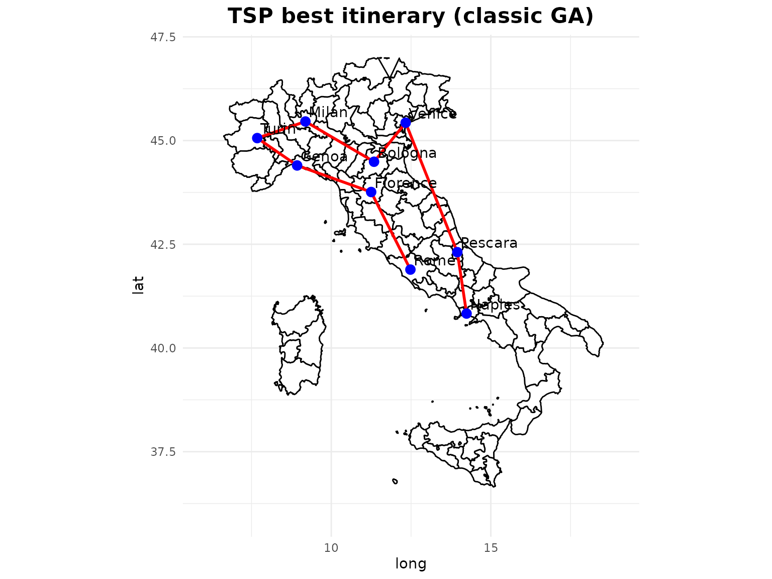
#> [1] "Rome"     "Florence" "Genoa"    "Turin"    "Milan"    "Bologna"  "Venice"   "Pescara"  "Naples"
cities_tsp <- cities[bestSolution,]
The sum of distances:
l = 0.0
for (i in 2:length(bestSolution)) {
  l = l+distance[bestSolution[i-1], bestSolution[i]]
}
l = l + distance[bestSolution[1],bestSolution[length(bestSolution)]]
l
#> [1] 18.42261
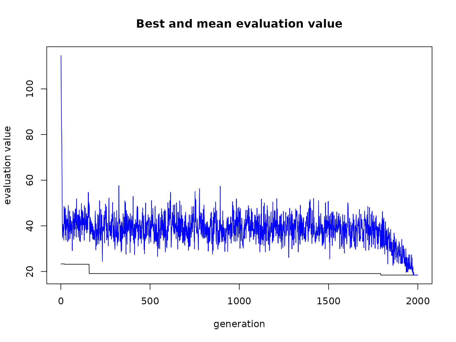
The fitness of the GA solution is lower than the one by the QGA.
italy_map <- map_data("italy")
lines <- data.frame(
  x = cities_tsp$x[-nrow(cities_tsp)],
  y = cities_tsp$y[-nrow(cities_tsp)],
  xend = cities_tsp$x[-1],
  yend = cities_tsp$y[-1]
)
gg <- ggplot() +
  geom_polygon(data = italy_map, aes(x = long, y = lat, group = group),
               fill = "white", color = "black") +
  geom_segment(data = lines, aes(x = x, y = y, xend = xend, yend = yend),
               color = "red", size = 1) +
  geom_point(data = cities_tsp, aes(x = x, y = y), color = "blue", size = 3) +
  geom_text(data = cities_tsp, aes(x = x, y = y, label = city),
            hjust = 0, vjust = 0, nudge_x = 0.1, nudge_y = 0.1) +
  coord_fixed(1.3) +
  theme_minimal() +
  ggtitle("TSP best itinerary (classic GA)") +
  theme(plot.title = element_text(hjust = 0.5, size = 16, face = "bold")) +
  xlim(6, 19) + ylim(36, 47)
print(gg)
Conclusions
In this case, the performance of the QGA is equivalent than the one of the classical GA (but the number of iterations of GA is the double).
Honestly, it has to be said that, increasing the number of the cities, GA outperforms QGA in the Traveller Salesman Problem.
In general, when the number of values that each element in the genome can assume is not high (in this case, we have 9 different values), then a relative efficiency of the QGA is to be expected. When the number of these values is higher, the classical GA tends to be more efficient.
This is because the QGA needs to define a number of qubits that is the integer ceiling value of log(n) (in our case n=9, so the number of required qubits is 3). The length of the solution is given by the product of the length of the genome (in our case 9) by the number of qubits necessary for each element of the genome.
In the particular case of the TSP, the greater length of the solution penalizes the QGA in the management of the solutions that present the same city more than once.