R2BEAT Optimization of precision constraints
2026-06-09
Source: vignettes/CVs_optimization.Rmd
CVs_optimization.Rmd
library(R2BEAT)
library("genalg")
library(kableExtra)
Introduction
In a multivariate stratified sampling design procedure, very often the values of the precision constraints (expressed in terms of maximum expected coefficients of variation set on the target estimates) are set taking into account the budget constraints that oblige to a given affordable sample size. This implies that an expert has to fine tune the precision constraints (increasing and decreasing them) until a satisfactory set is determined. When the number of variables and/or domains is not small, this job can be very expensive. To handle this issue, a new function, the “pareto” one, has been developed, in order to determine an optimal solution in terms of precision constraints, given the affordable sample size.
Another issue is related to the characteristics of the allocation of sampling units in the strata: it may happen that it can be very different from the proportional one. In some cases it may be desirable to limit the distance between the two allocations, avoiding the cases of too much oversampling in small strata. It is possible to obtain this, also in this case by changing the precision constraints. To get this result, it is possible to make use of a genetic algorithm, that explores the space of the possible combinations of values of the precision constraints, with the aim of maximizing the coefficient of correlation of the two distributions (optimal and proportional allocations).
Setting
In this study, we assume that the affordable sample size (given the budget) is set to 50,000. We show how it is possible to start from a “neutral” set of precision constraints (equal CVs for all variables for a given domain level), and modify them, so to:
first, balance the influence of all the variables on the determination of the best allocation, or at least, to avoid that only a small fraction plays a role;
secondly, get the optimal allocation closer to the proportional one.
We consider a strata dataframe containing information on labor force in a country. Each stratum belongs to three different domain levels:
load("strata.RData")
# strata$DOM3 <- NULL  # de-comment if you want to execute on 2 domains
str(strata)
## 'data.frame': 24 obs. of 18 variables:
## $ STRATUM : chr "north_1_3" "north_1_4" "north_1_5" "north_1_6" ...
## $ stratum_label: chr "north_1_3" "north_1_4" "north_1_5" "north_1_6" ...
## $ DOM1 : chr "National" "National" "National" "National" ...
## $ DOM2 : Factor w/ 3 levels "north","center",..: 1 1 1 1 1 1 1 1 2 2 ...
## $ N : num 92780 105327 200757 53612 102907 ...
## $ M1 : num 0.748 0.776 0.782 0.776 0.757 ...
## $ M2 : num 0.227 0.203 0.199 0.203 0.21 ...
## $ M3 : num 0.0252 0.0214 0.0192 0.0211 0.0329 ...
## $ M4 : num 29464 29364 27095 25726 27749 ...
## $ S1 : num 0.434 0.417 0.413 0.417 0.429 ...
## $ S2 : num 0.419 0.402 0.399 0.402 0.407 ...
## $ S3 : num 0.157 0.145 0.137 0.144 0.178 ...
## $ S4 : num 29839 27542 23575 19557 24520 ...
## $ CENS : num 0 0 0 0 0 0 0 0 0 0 ...
## $ COST : num 1 1 1 1 1 1 1 1 1 1 ...
## $ alloc : num 360 377 682 191 455 373 759 440 181 233 ...
## $ SOLUZ : num 352 368 667 187 444 365 742 431 177 227 ...
## $ DOM3 : chr "north_1_3" "north_1_4" "north_1_5" "north_1_6" ...We consider as target variables:
target_vars <- c("active","inactive","unemployed","income_hh")
target_vars
## [1] "active" "inactive" "unemployed" "income_hh"We initially set the following precision constraints:
# De-comment if you want to execute on 2 domains
# cv_equal <- as.data.frame(list(DOM = c("DOM1","DOM2"),
#                          CV1 = c(0.05,0.05),
#                          CV2 = c(0.05,0.05),
#                          CV3 = c(0.05,0.05),
#                          CV4 = c(0.05,0.05)))
# De-comment if you want to execute on 3 domains
cv_equal <- as.data.frame(list(DOM = c("DOM1","DOM2","DOM3"),
                         CV1 = c(0.05,0.05,0.05),
                         CV2 = c(0.05,0.05,0.05),
                         CV3 = c(0.05,0.05,0.05),
CV4 = c(0.05,0.05,0.05)))| DOM | CV1 | CV2 | CV3 | CV4 |
|---|---|---|---|---|
| DOM1 | 0.05 | 0.05 | 0.05 | 0.05 |
| DOM2 | 0.05 | 0.05 | 0.05 | 0.05 |
| DOM3 | 0.05 | 0.05 | 0.05 | 0.05 |
and proceed with an initial allocation:
equal <- R2BEAT::beat.1st(strata,cv_equal)with the following total sample size:
## [1] 137129Modification of the initial precision constraints to be compliant to the sample size constraint
We now change the initial precision constraints to reach the desired sample size.
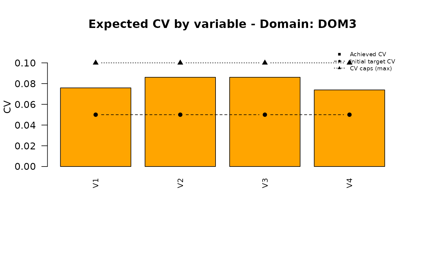
To this aim, we make use of the function ‘pareto’. This function determines an optimal set of precision constraints, compliant with the constraint in term of sample size.
Prior to the execution, we set some upper limits to the resulting precision constraints:
caps <- data.frame(
  DOM = c("DOM3"),
  VAR = c("V1","V2","V3","V4"),
  MAX_CV = c(0.10,0.10,0.10,0.10)
)
caps
## DOM VAR MAX_CV
## 1 DOM3 V1 0.1
## 2 DOM3 V2 0.1
## 3 DOM3 V3 0.1
## 4 DOM3 V4 0.1In this way, we indicate that whatever solution of the “pareto” function must be such that in DOM3 no CV can exceed these values.
out <- pareto(
  strata = strata,
  current_cvs = cv_equal,
  target_size = 50000,
  tolerance = 5,
  cv_caps = caps,
  beat1cv_fun = beat.1cv_2,
  max_iter = 50,
  max_same_iter = 20,
  plot = TRUE,
  plot_dir = "outputs",
  plot_prefix = "domains",
  show_targets = TRUE,
  show_caps = TRUE
)
## Start: t=1.0000000000 -> n=137129
## Bracket-up: t=1.2500000000 -> n=91446
## Bracket-up: t=1.5625000000 -> n=60184
## Bracket-up: t=1.9531250000 -> n=39246
## --> Bracket found (t_lo=1.0000000000 infeasible, t_hi=1.9531250000 feasible)
## Bisect 01: t=1.476562500000 -> n=66988
## Bisect 02: t=1.714843750000 -> n=50407
## Bisect 03: t=1.833984375000 -> n=44309
## Bisect 04: t=1.774414062500 -> n=47213
## Bisect 05: t=1.744628906250 -> n=48769
## Bisect 06: t=1.729736328125 -> n=49578
## Bisect 07: t=1.722290039062 -> n=49988
## Bisect 08: t=1.718566894531 -> n=50195
## Bisect 09: t=1.720428466797 -> n=50093
## Bisect 10: t=1.721359252930 -> n=50041
## Bisect 11: t=1.721824645996 -> n=50015
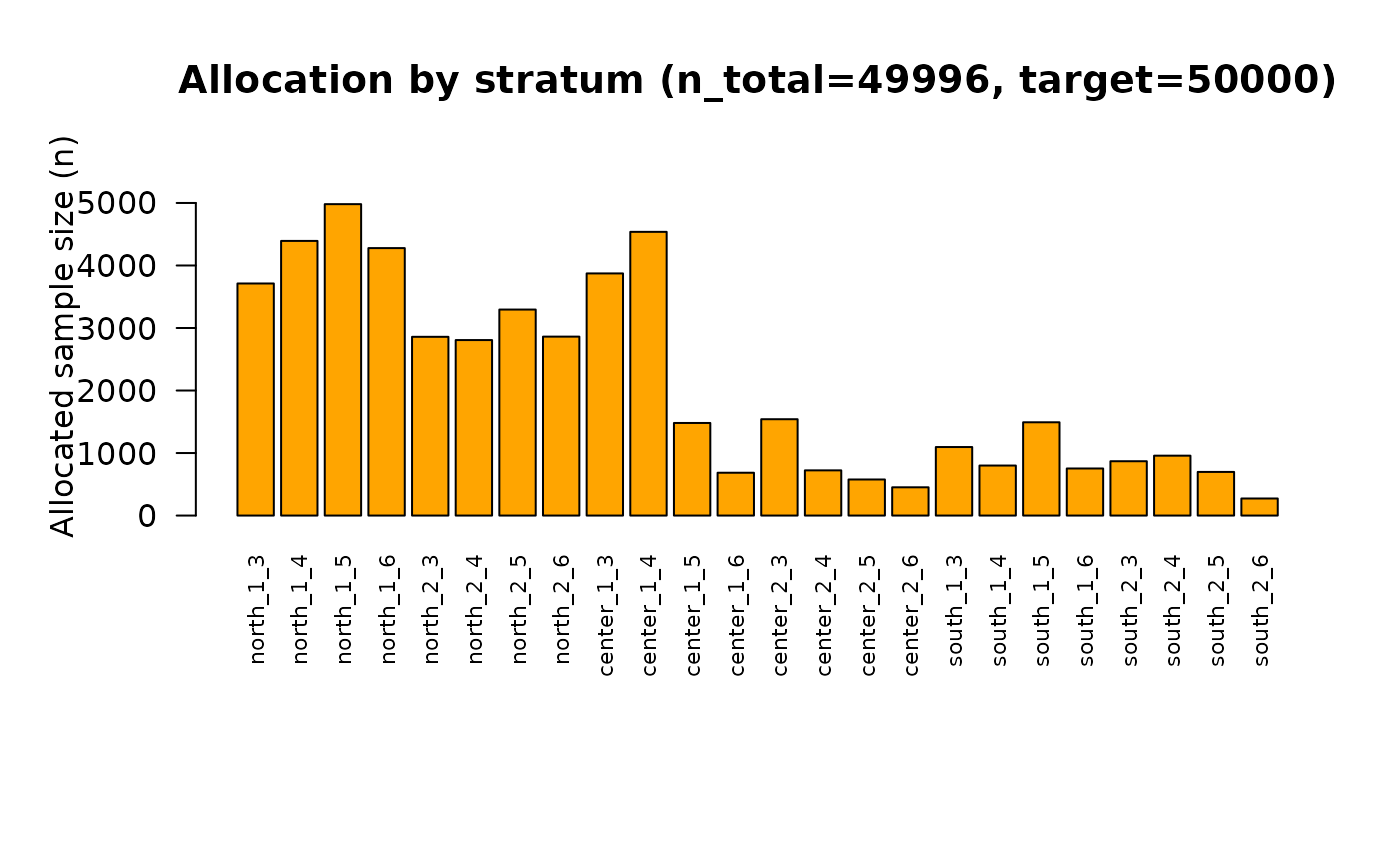
## Bisect 12: t=1.722057342529 -> n=50000## PNG saved: /home/runner/work/R2BEAT/R2BEAT/vignettes/outputs/domains_nmax_50000_tol_5_t_1.722057_convergence.png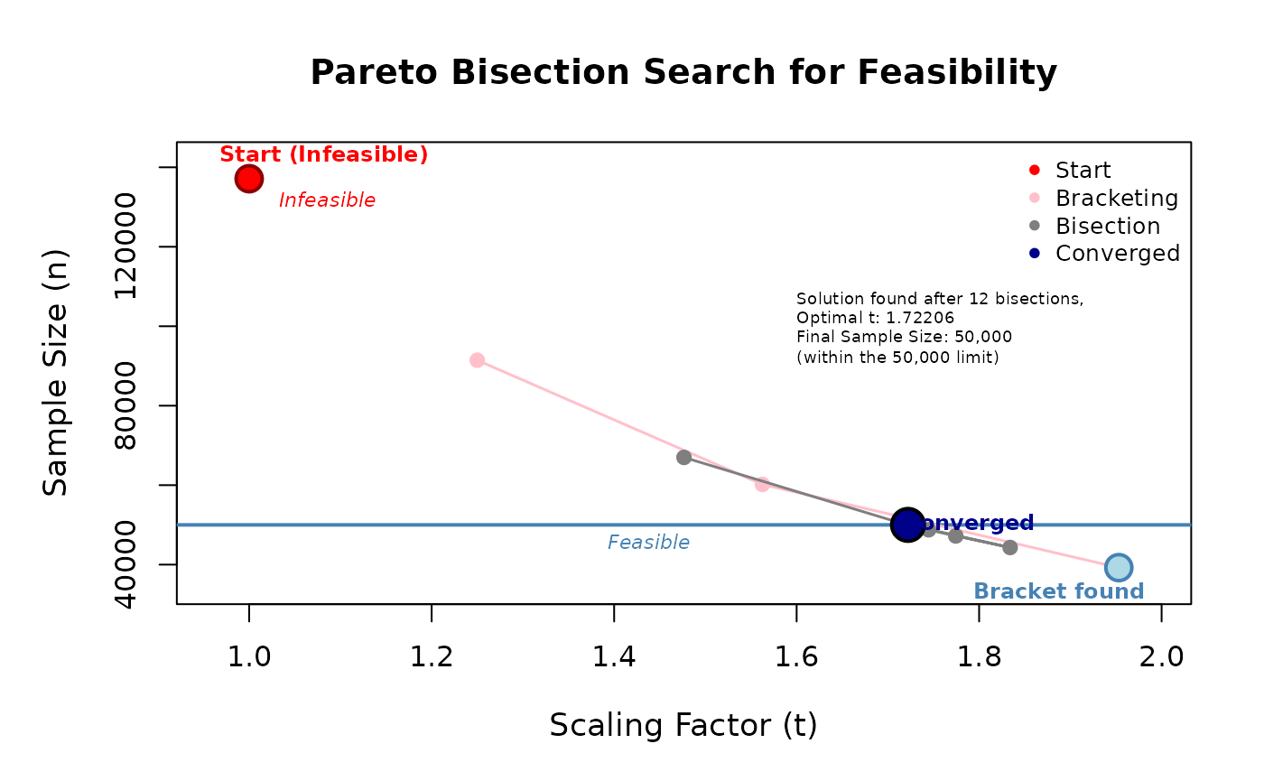


## PNG saved: /home/runner/work/R2BEAT/R2BEAT/vignettes/outputs/domains_nmax_50000_tol_5_t_1.722057_allocation.png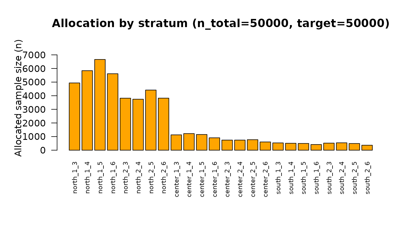
## PDF saved: /home/runner/work/R2BEAT/R2BEAT/vignettes/outputs/domains_CV_and_alloc_nmax_50000_tol_5_t_1.722057342529.pdfNow, the sample size is in line with the budget constraint:
sum(out$allocation$n)## [1] 50000These are the new CVs:
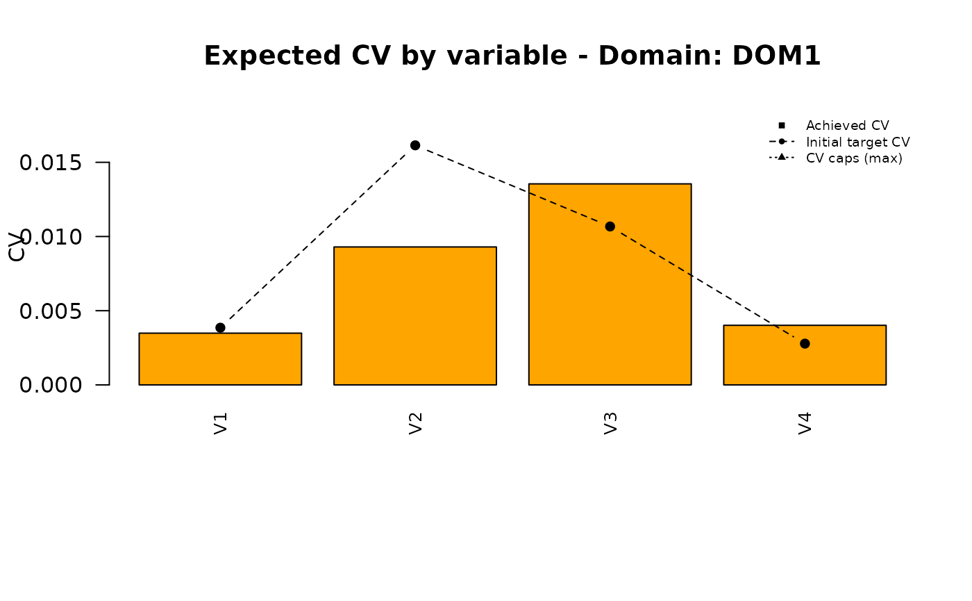
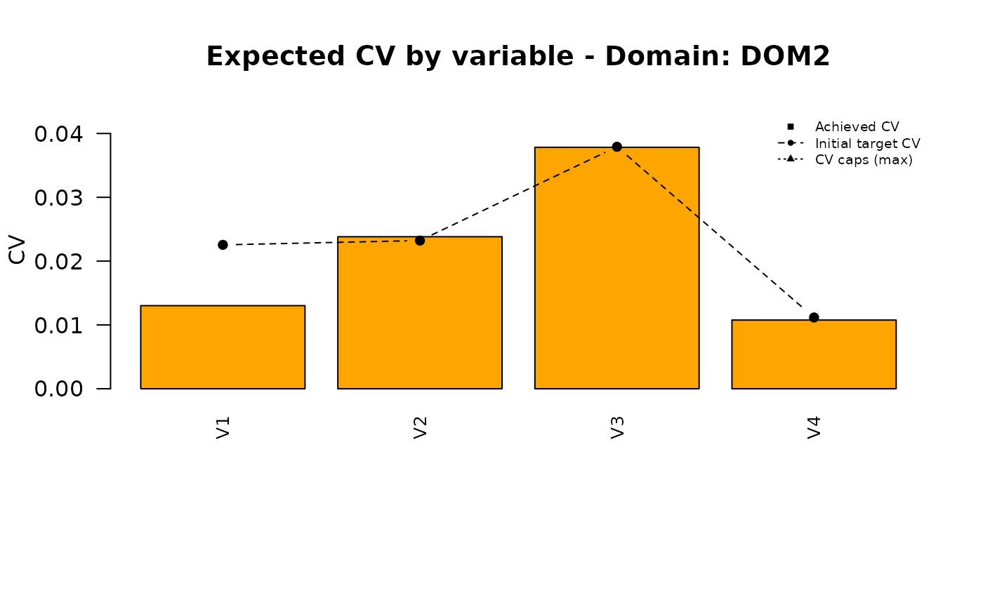
cv_pareto <- out$expectedCV
colnames(cv_pareto)[2:ncol(cv_pareto)] <- paste0("CV",c(1:ncol(cv_pareto)))
write.table(cv_pareto,"./outputs/2.pareto_cvs.csv",sep=",",quote=F,row.names=F)| DOM | CV1 | CV2 | CV3 | CV4 |
|---|---|---|---|---|
| DOM1 | 0.005 | 0.013 | 0.020 | 0.006 |
| DOM2 | 0.019 | 0.034 | 0.037 | 0.015 |
| DOM3 | 0.076 | 0.086 | 0.086 | 0.074 |
Get the optimal allocation closer to the proportional one
Consider the last obtained solution:
pareto_alloc <- beat.1st(strata,cv_pareto)
knitr::kable(
  pareto_alloc$alloc,
  digits = 3,
  caption = "Pareto allocation",
  format = "html"
) |>
  kableExtra::kable_styling(
    bootstrap_options = c("striped", "condensed"),
    full_width = FALSE
)| STRATUM | ALLOC | PROP | EQUAL | |
|---|---|---|---|---|
| north_1_3 | north_1_3 | 4938 | 2091.890 | 2083.417 |
| north_1_4 | north_1_4 | 5840 | 2374.785 | 2083.417 |
| north_1_5 | north_1_5 | 6661 | 4526.424 | 2083.417 |
| north_1_6 | north_1_6 | 5614 | 1208.778 | 2083.417 |
| north_2_3 | north_2_3 | 3819 | 2320.222 | 2083.417 |
| north_2_4 | north_2_4 | 3743 | 1891.698 | 2083.417 |
| north_2_5 | north_2_5 | 4416 | 4121.281 | 2083.417 |
| north_2_6 | north_2_6 | 3822 | 2249.741 | 2083.417 |
| center_1_3 | center_1_3 | 1127 | 4437.004 | 2083.417 |
| center_1_4 | center_1_4 | 1220 | 5871.453 | 2083.417 |
| center_1_5 | center_1_5 | 1152 | 2556.196 | 2083.417 |
| center_1_6 | center_1_6 | 910 | 352.947 | 2083.417 |
| center_2_3 | center_2_3 | 743 | 2278.037 | 2083.417 |
| center_2_4 | center_2_4 | 743 | 1060.510 | 2083.417 |
| center_2_5 | center_2_5 | 772 | 668.986 | 2083.417 |
| center_2_6 | center_2_6 | 605 | 563.331 | 2083.417 |
| south_1_3 | south_1_3 | 536 | 1377.992 | 2083.417 |
| south_1_4 | south_1_4 | 509 | 1664.088 | 2083.417 |
| south_1_5 | south_1_5 | 496 | 3097.838 | 2083.417 |
| south_1_6 | south_1_6 | 416 | 1286.587 | 2083.417 |
| south_2_3 | south_2_3 | 520 | 1238.405 | 2083.417 |
| south_2_4 | south_2_4 | 543 | 932.580 | 2083.417 |
| south_2_5 | south_2_5 | 492 | 1596.560 | 2083.417 |
| south_2_6 | south_2_6 | 365 | 234.667 | 2083.417 |
| Total | 50002 | 50002.000 | 50002.000 |
We can calculate the Pearson correlation coefficient between the optimal and proportional allocations:
cor(pareto_alloc$alloc$ALLOC[-nrow(pareto_alloc$alloc)],pareto_alloc$alloc$PROP[-nrow(pareto_alloc$alloc)])## [1] 0.3467993We want to get the optimal allocation closer to the proportional one. For instance, we want that the correlation coefficient be increased to 0.95.
To obtain this result, we make use of a particular genetic algorithm, the quantum genetic algorithm, implemented in the R package ‘genalg’.
First, we define the following fitness function:
fitness_cvs <- function(solution) {
  limit <- 0.95   #Insert here the desired correlation
  n_dom <- nrow(cv_pareto)
  n_vars <- ncol(cv_pareto) - 1
  if (length(solution) != n_dom * n_vars) {
    stop("solution length does not match n_dom * n_vars")
  }
  m <- matrix(solution, nrow = n_dom, ncol = n_vars, byrow = TRUE)
  cv_corr <- data.frame(
    DOM = paste0("DOM", 1:n_dom),
    m
  )
  colnames(cv_corr)[2:(n_vars + 1)] <- paste0("CV", 1:n_vars)
  cv_corr
  a <- R2BEAT::beat.1st(strata,cv_corr)
  # b <- ks.test(a$alloc$ALLOC[-nrow(a$alloc)],a$alloc$PROP[-nrow(a$alloc)])
  c <- cor(a$alloc$ALLOC[-nrow(a$alloc)],a$alloc$PROP[-nrow(a$alloc)])
  #---------- Fitness function ----------------
  if (abs(c) > limit + 0.005) c <- 0
  fitness <- -c # genalg always minimizes, so we invert the sign
  return(fitness)
}
The, we set the parameters required by the optimization function (rbga):
nvars <- ncol(cv_pareto) - 1
vett <- NULL
for (k in c(1:nrow(cv_pareto))) {
  vett <- c(vett,cv_pareto[k,c(2:(nvars+1))])
}
vett <- unlist(vett)
vettmin <- vett * 0.5
vettmax <- vett * 1.5
Some explanations regarding the parameters. The parameters ‘vettmin’ and ‘vettmax’ are fundamental to determine the space of possible solutions.
In fact, consider their values:
vettmin## CV1 CV2 CV3 CV4 CV1 CV2 CV3 CV4
## 0.0024570 0.0064705 0.0099120 0.0027510 0.0094300 0.0172095 0.0186080 0.0076745
## CV1 CV2 CV3 CV4
## 0.0379405 0.0430485 0.0430515 0.0369505
vettmax## CV1 CV2 CV3 CV4 CV1 CV2 CV3 CV4
## 0.0073710 0.0194115 0.0297360 0.0082530 0.0282900 0.0516285 0.0558240 0.0230235
## CV1 CV2 CV3 CV4
## 0.1138215 0.1291455 0.1291545 0.1108515The values in vettmin are the minimum values that the CVs can assume, while the values in vettmax are the maximum ones.
NOTE: the higher the difference between the current correlation and the desired one, the wider the acceptable intervals of variation of the CVs: in this case we assumed plus and minus 50% for each CV.
set.seed(1234)
solution_genalg <- rbga(stringMin=vettmin,
                        stringMax=vettmax,
                        evalFunc=fitness_cvs,
                        popSize=10,
                        iters=50)
ndoms = nrow(cv_pareto)
par(mfrow=c(1,2))
#plot vett
plot(vett, col="black", type="l",xaxt = "n", ylim=c(min(vettmin), max(vettmax)), xlab="", ylab="", main="Region of variation for CVs") # xaxt = "n" disables the xaxis ticks
# Generate the vector of labels
vector_labels <- paste("DOM", rep(1:ndoms, each = nvars),
                       "_V", rep(1:nvars, times = ndoms),
                       sep = "")
# xticks
axis(side=1,at=seq(1,length(vett)),labels=vector_labels, las=2, cex.axis=0.5)
# vettmin and vettmax
lines(vettmin, col="red")
lines(vettmax, col="blue")
# add legend
legend("topleft", legend=c("cv_input", "cv_min", "cv_max"), col = c("black", "red", "blue"), lty=1, cex=0.5)
plot(solution_genalg)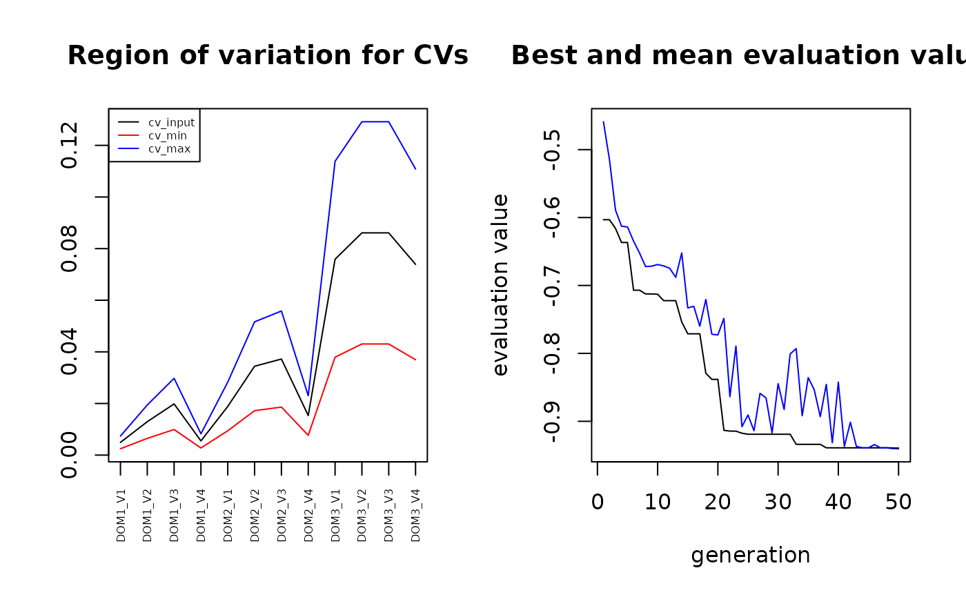
This is the obtained correlation coefficient:
-min(solution_genalg$evaluations)## [1] 0.9404242We decode the found solution:
filter = solution_genalg$evaluations == min(solution_genalg$evaluations)
if (sum(filter) > 1) bestSolution = solution_genalg$population[filter, ][1,]
if (sum(filter) == 1) bestSolution = solution_genalg$population[filter, ]
bestSolution
## [1] 0.003854673 0.016145110 0.010674814 0.002781292 0.022548258 0.023220772
## [7] 0.037919427 0.011165544 0.109226446 0.120572356 0.124485601 0.108484576
m <- matrix(bestSolution, nrow = ndoms, ncol = nvars, byrow = TRUE)
cv_ga <- data.frame(
  DOM = paste0("DOM", 1:ndoms),
  m
)
colnames(cv_ga)[2:ncol(cv_ga)] <- paste0("CV", 1:nvars)| DOM | CV1 | CV2 | CV3 | CV4 |
|---|---|---|---|---|
| DOM1 | 0.004 | 0.016 | 0.011 | 0.003 |
| DOM2 | 0.023 | 0.023 | 0.038 | 0.011 |
| DOM3 | 0.109 | 0.121 | 0.124 | 0.108 |
## [1] 91710
cor(ga_solution$alloc$ALLOC[-nrow(ga_solution$alloc)], ga_solution$alloc$PROP[-nrow(ga_solution$alloc)])## [1] 0.9404242Re-execution of the “pareto” function
With these new precision constraints, the sample size is greater than the affordable. So, we apply again the “pareto” function:
out2 <- pareto(
  strata = strata,
  current_cvs = cv_ga,
  target_size = 50000,
  tolerance = 5,
  cv_caps = caps,
  beat1cv_fun = beat.1cv_2,
  max_iter = 50,
  max_same_iter = 20,
  plot = TRUE,
  plot_dir = "outputs",
  plot_prefix = "domains",
  show_targets = TRUE,
  show_caps = TRUE
)
## Start: t=1.0000000000 -> n=92650
## Bracket-up: t=1.2500000000 -> n=62120
## Bracket-up: t=1.5625000000 -> n=45830
## --> Bracket found (t_lo=1.0000000000 infeasible, t_hi=1.5625000000 feasible)
## Bisect 01: t=1.281250000000 -> n=59627
## Bisect 02: t=1.421875000000 -> n=50976
## Bisect 03: t=1.492187500000 -> n=48079
## Bisect 04: t=1.457031250000 -> n=49430
## Bisect 05: t=1.439453125000 -> n=50176
## Bisect 06: t=1.448242187500 -> n=49797
## Bisect 07: t=1.443847656250 -> n=49985
## Bisect 08: t=1.441650390625 -> n=50082
## Bisect 09: t=1.442749023438 -> n=50033
## Bisect 10: t=1.443298339844 -> n=50010
## Bisect 11: t=1.443572998047 -> n=49996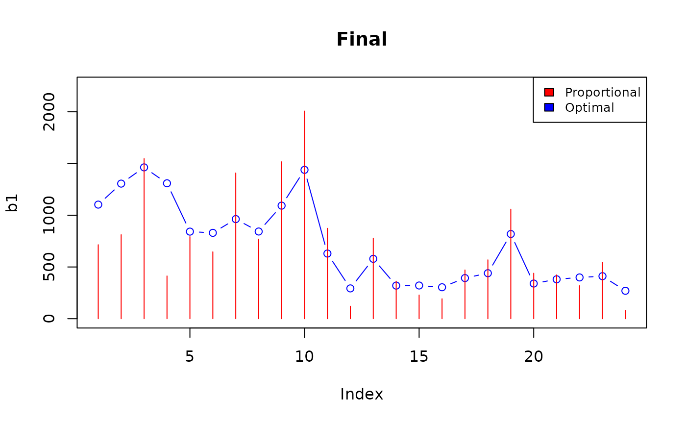

Analysis of the final solution
These is the final set of precision constraints:
| DOM | CV1 | CV2 | CV3 | CV4 |
|---|---|---|---|---|
| DOM1 | 0.006 | 0.023 | 0.015 | 0.004 |
| DOM2 | 0.033 | 0.034 | 0.055 | 0.016 |
| DOM3 | 0.100 | 0.100 | 0.100 | 0.100 |
that produces the following sample size:
## [1] 49996in line with the affordable sample size.
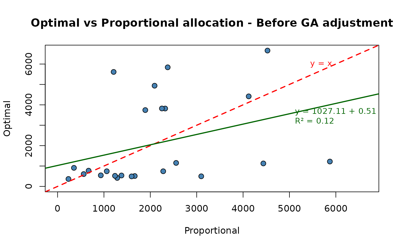
What about the closeness of the final optimal allocation to the proportional one?
df <- pareto_alloc$alloc
df <- df[-nrow(df),]
rng = c(0, max(df$ALLOC,df$PROP))
p1 <- plot(ALLOC  ~  PROP,
     data = df,
     main = "Optimal vs Proportional allocation - Before GA adjustment",
     ylab = "Optimal",
     xlab = "Proportional",
     xlim = rng,
     ylim = rng,
     pch = 21,
     bg  = "steelblue",
     col = "black",
     cex = 1.2)
abline(a = 0, b = 1, col = "red", lwd = 2, lty = 2)
text(
  x = rng[2] * 0.8,
  y = rng[2] * 0.9,
  labels = "y = x",
  col = "red",
  pos = 4,
  cex = 0.9
)
fit <- lm(ALLOC~PROP, data = df)
coefs <- coef(fit)
r2 <- summary(fit)$r.squared
abline(fit, col = "darkgreen", lwd = 2)
text(
  x = rng[2] * 0.75,
  y = rng[2] * 0.5,
  labels = sprintf("y = %.2f + %.2f x\nR² = %.2f",
                   coefs[1], coefs[2], r2),
  col = "darkgreen",
  pos = 4,
  cex = 0.9
)
df <- final_sol$alloc
df <- df[-nrow(df),]
rng = c(0, max(df$ALLOC,df$PROP))
p2 <- plot(ALLOC ~ PROP,
data = df,
main = "Optimal vs Proportional allocation - After GA adjustment",
ylab = "Optimal",
xlab = "Proportional",
xlim = rng,
ylim = rng,
pch = 21,
bg = "steelblue",
col = "black",
cex = 1.2)
abline(a = 0, b = 1, col = "red", lwd = 2, lty = 2)
text(
x = rng[2] * 0.8,
y = rng[2] * 0.9,
labels = "y = x",
col = "red",
pos = 4,
cex = 0.9
)
fit <- lm(ALLOC~PROP, data = df)
coefs <- coef(fit)
r2 <- summary(fit)$r.squared
abline(fit, col = "darkgreen", lwd = 2)
text(
x = rng[2] * 0.75,
y = rng[2] * 0.5,
labels = sprintf("y = %.2f + %.2f x\nR² = %.2f",
coefs[1], coefs[2], r2),
col = "darkgreen",
pos = 4,
cex = 0.9
)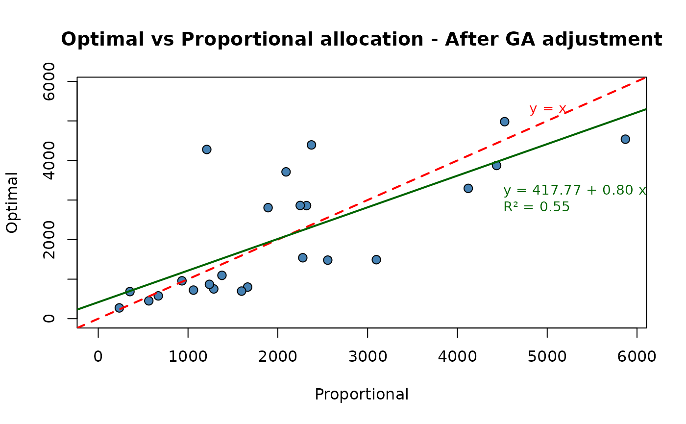 So, we obtained a final optimal solution that is much more close to the
proportional one with respect to the one obtained with the first
application of the “pareto” function.
So, we obtained a final optimal solution that is much more close to the
proportional one with respect to the one obtained with the first
application of the “pareto” function.
It is worth noting that the final correlation:
## [1] 0.7391439is not the one that we indicated to and obtained by the genetic algorithm. This is due to the fact that when re-applying the “pareto” function, we lost some of the correlation. If we want a higher value of it we should get back to the genetic algorithm and set a higher value for the desired correlation.
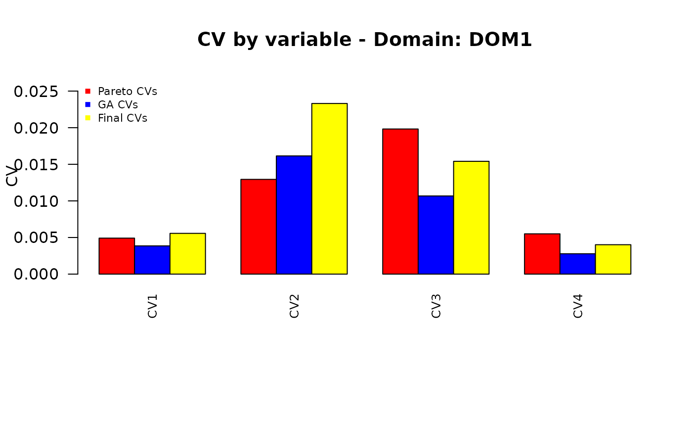
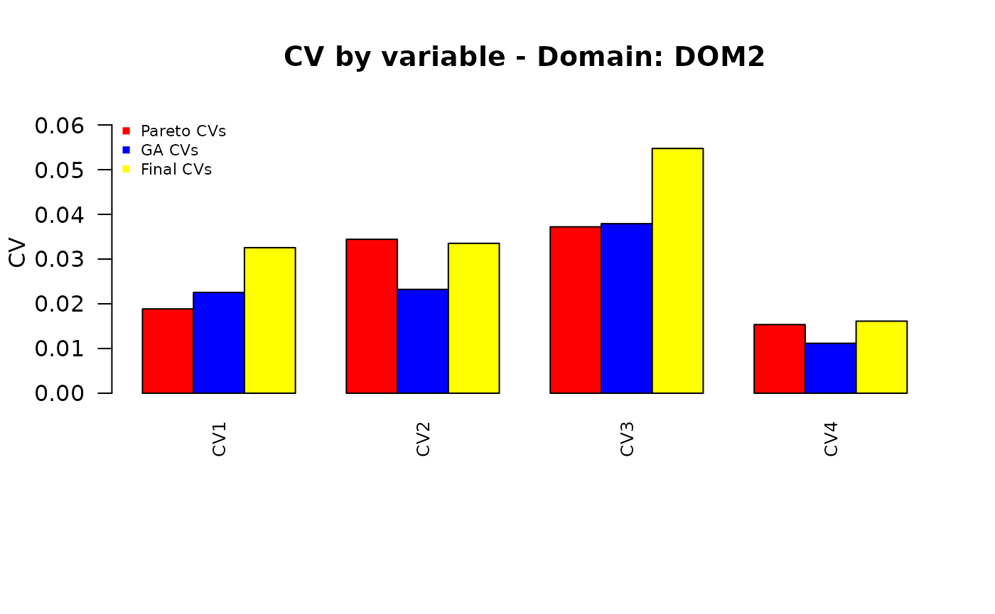
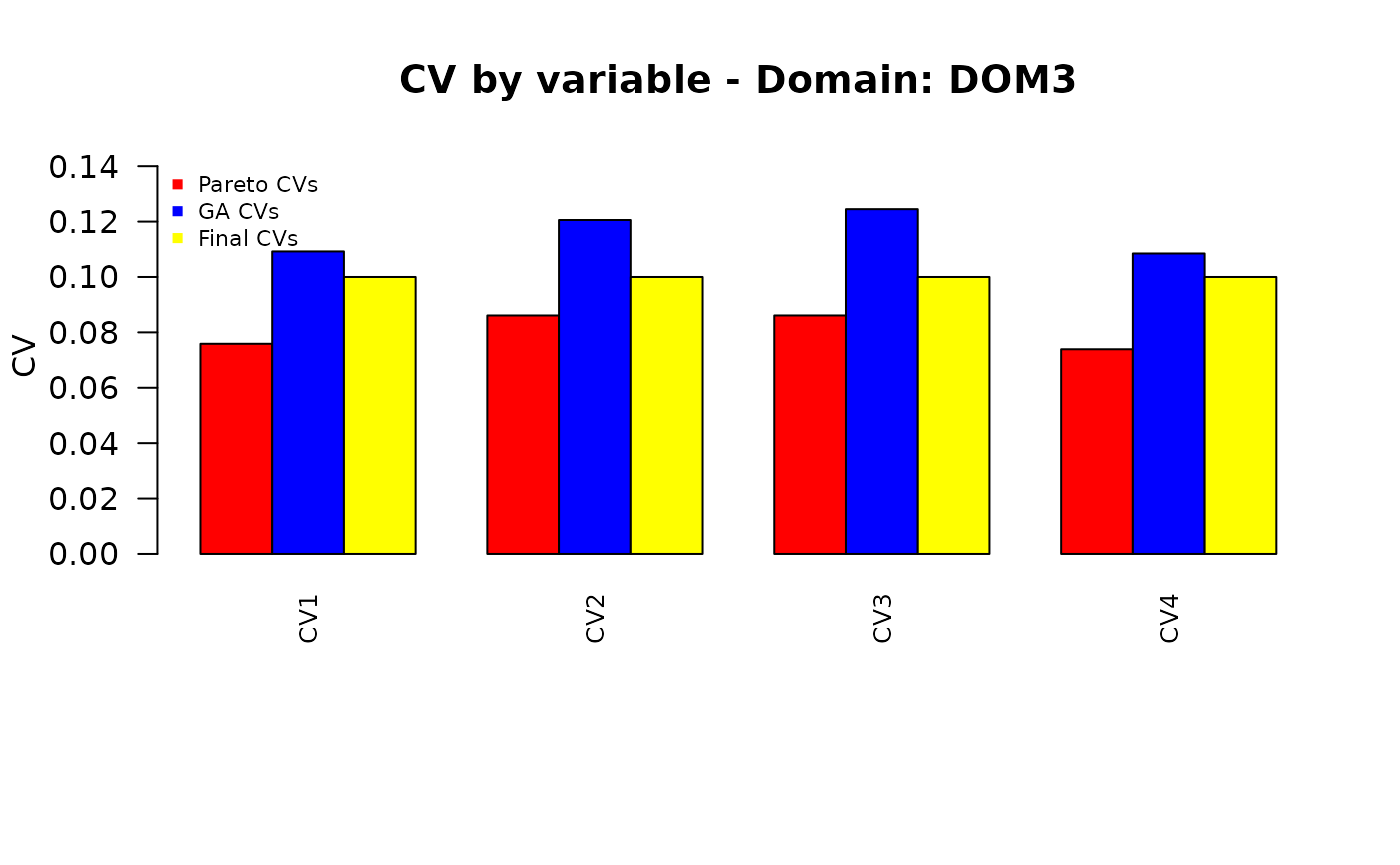
Finally, we want to compare the different sets of the precision constraints:
those obtained by applying the “pareto” function to the set of equal CVs;
those obtained by applying the genetic algorithm;
the final ones, obtained by re-applying the “pareto” function.
plot_domain <- function(dom_label, cv_pareto, cv_ga, cv_final,
                        series_cols = c("red", "blue","yellow")) {

  vnames <- names(cv_pareto)

  op <- par(no.readonly = TRUE)
  on.exit(par(op), add = TRUE)
  par(mar = c(8, 4, 4, 2) + 0.1)

  ymax <- max(cv_pareto, cv_ga, cv_final, na.rm = TRUE) * 1.15

  heights <- rbind(Pareto = cv_pareto, GA = cv_ga, Final = cv_final)

  bp <- barplot(
    heights,
    beside = TRUE,
    names.arg = vnames,
    las = 2,
    cex.names = 0.8,
    ylim = c(0, ymax),
    main = paste("CV by variable - Domain:", dom_label),
    ylab = "CV",
    col  = series_cols
  )

  # bp è una matrice 2 x nvar con le x dei bar; prendiamo i centri del gruppo
  x_centers <- colMeans(bp)

  # linea tratteggiata (cv_ga)
  # lines(x_centers, ga_vals, type = "b", lty = 2, pch = 16)

  legend(
    "topleft",
    legend = c("Pareto CVs", "GA CVs", "Final CVs"),
    col    = c(series_cols),
    pch    = c(15, 15, 15),
    bty    = "n",
    cex = 0.7
  )
}


doms <- unique(cv_pareto$DOM)
ncols <- ncol(cv_pareto)
vcols <- names(cv_pareto)[2:ncol(cv_pareto)]

for (d in doms) {
  pareto_row     <- cv_pareto[cv_pareto$DOM  == d, vcols, drop = FALSE]
  ga_row <- cv_ga[cv_ga$DOM == d, vcols, drop = FALSE]
  final_row     <- cv_final[cv_final$DOM  == d, vcols, drop = FALSE]

  if (nrow(pareto_row) != 1 || nrow(ga_row) != 1 || nrow(final_row) != 1) {
    warning("Dominio ", d, ": righe non univoche nei file. Salto.")
    next
  }

  pareto_vals <- as.numeric(pareto_row[1, ])
  ga_vals     <- as.numeric(ga_row[1, ])
  final_vals     <- as.numeric(final_row[1, ])

  names(pareto_vals) <- names(ga_vals) <- names(final_vals) <- vcols
  plot_domain(dom_label = d, cv_pareto = pareto_vals, cv_ga = ga_vals, cv_final = final_vals)
}